Decisions on the expansion and contraction of product lines form a major component of a company’s forward strategy. It is a focal point at which policy on production, marketing and distribution must be jointly co-ordinated. Typically, this type of planning is undertaken on a yearly basis and is linked to the annual budget proposals. The procedures for deciding product plans may vary from an exact objective approach using forward estimates to schemes for coping with current difficulties and alleviating the immediate procedures on marketing, production or financial staff. However, as quantitative techniques become more common in management and more detailed data becomes available, it is possible to employ formal computational models to assist with the forward planning task. This is the aim of the system which have been designed and called MAPLE for Marketing and Product Line Evaluation. It aims to provide a simple means of a company to enter data into a computer, to perform an optimising calculation and to point out typical planning and accounting information. The intention of the model is not just to indicate the best plan which could be adopted, but also to indicate the feasibility of proposed plans, to suggest the direction in which the promising changes could be made and to point out areas where further investigations should be carried out. Perhaps the most powerful role of the program is the commitment it provides to organise and analyse the company’s data to be used for planning and to provide a central but neutral point of reference for functional management who may tend to operate independently.

The system is planned on the basis of case investigations into what is needed in practice. Company control often extends across a number of production sites and a number of marketing zones and the system therefore envisages a multi-factory environment. The primary planning problem which a company faces is to decide how much of each product line should be manufactured at each production centre for each market sector. These decisions involve much more than finding the best product mix at a factory for given sales requirements, which is the traditional way in which linear programming has been used on this problem. Given the production process capacities we need to employ the resources efficiently, it is also necessary to plan how much to sell. The sales of the products can be influenced and controlled through the advertising and pricing policies. Further profit may depend on an ability to generate extra sales. On the other hand, if sales can be increased beyond base production capacities the question of employing extra, more costly capacity such overtime or sub-contracting must be examined. Moreover, with each of these possibilities the distribution costs must be considered. The MAPLE system, therefore, sets out to consider the policy decisions on production, marketing and distribution collectively. The planning or control variables in the system are therefore as follows:

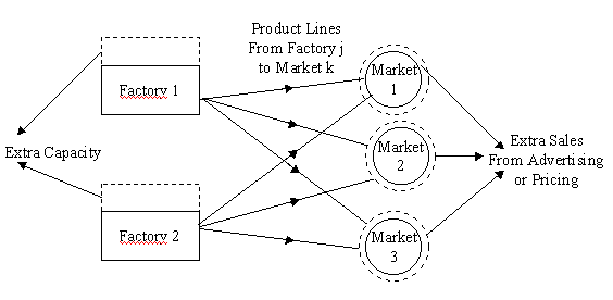
The first two types of variables are primarily production decisions and the latter two types are marketing decisions. (The composite first type of variable implies the distribution policy.) The scope of the system is illustrated in the figure 1 for two factories and three market sectors.

 

Figure 1 The scope of the system with two factories and three market sectors.

For the system to be practicable it is important that the user should not have to formulate company’s planning problem in mathematical terms. The data input to the system is therefore arranged in a set of files of data items which are directly related to this planning problem. In order to apply the system it is only necessary to select the data items from the production, marketing and accounting records and fit them into the required slots. The principle data items contained in the six files are outlined below.

All this data is now organised automatically inside the program into a linear programming form and the linear programming problem is solved by standard calculations. It is not possible to built prices into the formulation in a linear form; instead, the various possible price combinations are studied individually by taking each set of prices and obtaining a solution to the problem in terms of the product quantities, extra capacities and advertising. The search over the possible price combinations can be guided by the successive solutions to the linear programming problem.

To indicate the way in which the linear programming problem takes shape, we first define the problem variables as:

Next the objective expression is created which consists of a sum of terms in Xijk, Yim and Zi each variable being multiplied by a number of coefficient for Xijk is expressed as:

This expression for total variable profit is to be maximised subject to variety of constraints. The constraints are typically represented as in equalities. For instance, the total amount produced of product line i at all factories and distributed to market sector k must be less than the upper limit on demand at market sector k. The range of constraints include:

It is useful at this point to illustrate the procedure with a small example in which there are two factories, and two markets. It is easy to tackle this problem by visual inspection and some simple judgements, but its simplicity assists the understanding of the procedure. It should be stressed, however, that the MAPLE system applies to the much of wider content of many factories and many markets.

Suppose a firm is making four products A, B, C and D at two factories for two separate markets. Each of the products are made by compounding some materials and then passing the material through one of the two possible manufacturing processes. Product A and B go through process 1 and products C and D go through process 2. The material costs are given in Table 1.

Table 1 Material Costs

The variables production costs and capacities on the two processes are distinguished by regular time and overtime as shown in Table 2. The variable production costs would not normally include machine depreciation, but could well include power and other variable inputs and possibly also labour as it may well be possible to plan the size of the required labour force with the planning horizon set at one year.

Table 2 Variable production costs and capacities

Table 3 Price and demand alternative

The demand can also be influenced by advertising expenditure. The response to advertising varies depending on the product. The estimated percentage increase on the base demand for $10000 of advertising is shown in Table 4.

Table 4 Advertising response

There is a limit to the amount of money which can be spent on advertising. $70000 is the total advertising budget and there is a limit $10000 to be spent on advertising on product C.

All these data can be expressed in the linear programming formulation described in the previous section. Xijk values are 1000 tons, Yim values are 1000 tons and Zi values are $1000.

So the objective function is expressed as:

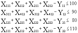
where for Xijk C111 = 20 = price (60) - material costs (32) - processing cost (8)

for Yjm C11 = 1.2 = regular time cost (8) - overtime cost (9.2)

The base capacity constraint on process 1 expresses the fact that the total production of products A and B, less the amount produced in overtime, must not be greater than 100000 tons. This and the other capacity constraints are expressed by the inequality

The advertising effect is reflected to the model by the following inequalities

Finally the advertising constraints require that

The linear programming problem can now be solved to give the solution shown in Table 5.

Table 5 Solution of the linear programming problem

The solution shows that it is not worth while to use overtime on the first process in the first factory and it is not worth of advertising on products A and C and the total advertising expenditure is taken up to the full limit.

The output from the system provides classified reports on the plans and a sensitivity analysis to indicate the effects of making changes on the constraints.

The basic output includes detailed reports on the following topics:

The linear programming solution also provides a valuable sensitivity analysis. Besides the basic results on the problem variables of production, distribution and marketing, the solution contains some quantities called simplex multipliers or shadow prices which give the change in profits that would result from altering any of the constraining values such as production capacities or market demands. The simplex multiplier for each constraint gives the marginal increase in profit for a unit change in the constraint. This is exactly the kind of information which is needed for a sensitivity analysis, and it is automatically provided without doing repeated runs on the programme.

The sensitivity analysis can also be helpful for assessing the effects of uncertainties in some of the data items. As the simplex multipliers indicate the rate of change of profit with change in a constraining value, it is clearly the quantities connected with the large simplex multipliers which need to be checked for accuracy and reliability. The further uncertainties in the data may be examined directly by running the programme with upper and lower limits on the data to check the sensitivity of the results in different circumstances.

The MAPLE system has been designed to provide a simple means for a company to consider applying quantitative methods to assist with their decisions on product planning. The data files of input which are planned specifically for this management area provide a scheme for the manager to recognise the scope of the system and enter data into the calculation to use the linear programming calculation. It means that once the data have been assembled the system can be run without any further time and money being spent on setting up a special computing project to solve the problem.

The file system envisages a general model for a multi-factory and multi-market situation and features within the programme can readily be altered to suit the special requirements of the individual companies once it appears that the scheme is relevant for their planning problems. Sometimes these extensions simply involve a re-interpretation of a data item. For instance, a factory may wish to distinguish its contracting out from its use of overtime as a source of extra capacity. This can be done by renaming the contracting out facility as a separate factory on the same site. Equally, if it is required to price a product differently into two distinct market sectors, the product can be differentiated on two separate products with the same production characteristics.

It is important for management to recognise the flexibility of the system. It should not be seen simply as a single linear programming calculation, but a general decision making model which can be used to explore numerous possible opportunities to the company. The output from programme does not dictate the annual plan which must be adopted but rather provides the basis for judgement across the three fields of production, marketing and distribution. The competition should be run regularly as a check on performance and as forecast on sales and updated in the light of changing circumstances.